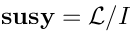
Vertex operators in AdS

and Koszul duality

Andrei Mikhailov, IFT UNESP

Based on http://arxiv.org/abs/1207.2441


Passa Quatro, August 2012

1 Introduction

Theoretical physics has traditionally been very close to geometry.

But more recently it appears that our mathematical guide should be algebra, not geometry. It seems that geometrical constructions (such as smooth manifold in its traditional definition) are an artifact of taking the classical limit. Quantum mechanics, on the other hand, is based on algebra.

It would seem that some theoretical physics constructions could become more useful if translated into algebraic language.

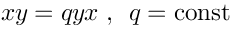
Algebraically speaking, what is smooth manifold? Smooth manifold can be identified as a commutative algebra, namely the algebra of functions on this manifold. For example is identified with the algebra formed by two letters and with the relation:

(1)

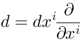
Now, we can deform this algebra. For example:

(2)

This is the noncommutative . We can ask ourselves how various geometrical constructions generalize to the noncommutative case.

In my talk I will discuss the technique which evolved around the noncommutative generalization of the de Rham differential. The commutative de Rham differencial is:

But what happens if we consider noncommutative ? How to generalize , and what would be its properties?

It turns out that this question is quite relevant to modern string worldsheet theory (Berkovits formalism).

2 Plan of the talk

1. Free algebras and algebras with quadratic relations

2. Koszul duality, Koszul differential

3. Relation to pure spinor formalism:

   1. Pure spinors as Koszul algebra

   2. BRST cohomology vs Lie algebra cohomology

   3. Application to vertex operators in AdS and flat space

3 Free algebras

Algebra is a linear space with a multiplication operation.

Example: tensor algebra, also called free algebra:

Take a linear space and consider the space of all (finite) linear combinations of expressions of the form:

   where  

The notation implies that and

This is called tensor algebra, and denoted

4 Quadratic algebras

Quadratic algebras are tensor algebras with quadratic relations. This means that we consider the factorspace:

(quadratic relations)

What does this mean? Let us introduce the basis in . Quadratic relations are defined by a set of constant matrices :

(3)

That is, all the expressions of the form are considered zero.

A standard notation for this algebra is:

5 Examples of quadratic algebras

Example 1: suppose that run over all antisymmetric matrices. In this case the resulting quadratic algebra is just the algebra of polynomials of variables, where , or equivalently the algebra of symmetric tensors. Another name for it is “symmetric algebra”:

(4)

---

Example 2: runs over all symmetric matrices. In this case is the exterior algebra :

(5)

This is the algebra of antisymmetric tensors.

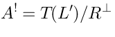
6 Dual algebra

We have just defined a quadratic algebra .

Now we will define the dual algebra, which is denoted .

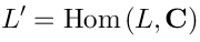
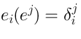
Consider the linear space which is dual to :

As we introduced the basis in , we can introduce the dual basis in . “Dual basis” means:
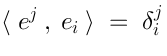
Remember that was defined using the set of constant matrices , which were used to define the quadratic constraints (3). Consider the linear space of all the matrices orthogonal to every . “Orthogonal” means that satisfies the equation:

(6)

Suppose that , is a set of linearly independent solutions of this equation. Let us consider:

(7)

where is generated by the tensors of the form:

Conclusion: We started from a quadratic algebra and constructed another quadratic algebra , which is called quadratic dual to .

7 Example of mutually dual algebras

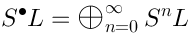
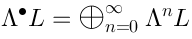
Example: We have already explained that the symmetric algebra and exterior algebra are particular cases of quadratic algebras. In fact, they are Koszul dual to each other:

(8)

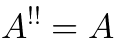
Notice that the operation of “Koszul duality” applied twice brings us back to :

In particular, we can also say:

(9)

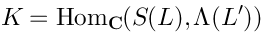
8 Koszul Complex

Consider the following space:

(10)

- the space of linear maps from to .

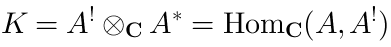
It turns out that naturally comes with some nilpotent operator , which is a noncommutative generalization of the de Rham complex.

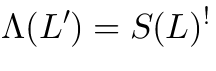
We will explain this using the particular example (8), (9) of dual algebras; in that particular case is exactly the de Rham differential.

9 De Rham complex

As a partucular example, let us consider , . In this case we get:

(11)

This is the de Rham complex for the flat space .

Explanation:

Our is an -dimensional vector space. Let us introduce a basis and call the basis elements :

(this is just a notation, just use letter instead of ). What is ? It is the space of polynomials of , i.e.:

(12)

And what is the dual space ? It is the space of “Taylor series”:

(13)

The dual space has the following basis:

(14)

Finally, what is ? Here it is:

(15)

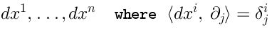
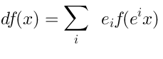
The De Rham differential acts as usual:

This operator is nilpotent. Moreover, it provides the resolution of in the sense that the following complex:

(16)

is exact.

Mathematically speaking, the de Rham complex provides:

An injective resolution of the module

10 Koszul complex

The general Koszul complex is a more or less direct generalization of this construction.

generalizes to

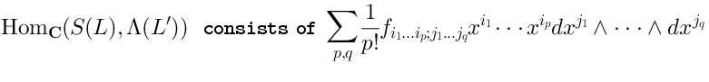
Elements of can be written as . We have to explain how acts on . For that we need to remember that and

Let us introduce a basis in and a dual basis in ; the “dual basis” means that:

We define:

(17)

One can see that

11 Koszul complex

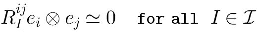
Notice that and are both graded algebras, therefore we can define , , . Consider the complex:

(18)

It consists of injective modules, but is it exact?

The question about exactness is a nontrivial one. It depends on .

Mathematicians have tools to address this question. (The theory of quadratic algebras.)

If (18) is exact, then the algebra is called a “Koszul algebra”. If is Koszul, then is also Koszul, and vise versa. Duality of quadratic algebras is symmetric.

12 Koszul duality and string theory

We will now turn to string theory.

Unfortunately I do not have time to discuss the Berkovits formalism for the Type IIB superstring theory.

If you know this formalism, you will recognize the structures which I will discuss.

If not, I will try to make sure that at least the general physical meaning be understandable.

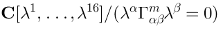
13 Pure spinors as a Koszul algebra

It turns out that the algebra of pure spinors in 10D:

(19)

is Koszul.

The dual algebra is the algebra of covariant derivatives of the 10-dimensional supersymmetric Yang-Mills theory:

(20)

It is therefore also Koszul.

We will denote:

(21)

In this case is the universal enveloping algebra:

(22)

where is the Lie algebra formed by nested commutators of the letters .

14 Koszul dual of a commutative algebra

General observation:

Consider the case when is a commutative algebra. This means that includes all antisymmetric tensors.

⇒

is a universal enveloping of a Lie algebra.

Example: If is the algebra of polynomials of variables , then the dual Lie algebra is the algebra of antisymmetric polynomials . This is the universal enveloping of the Lie superalgebra .

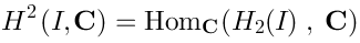
15 BRST complex and Lie algebra cohomology

Main idea

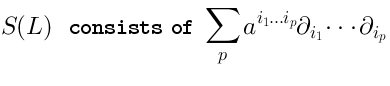
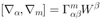
The BRST complex, as it arizes in the pure spinor string theory, involves a representation of the algebra (the algebra of covariant derivatives). The BRST operator acts on the space of functions of , taking values in :

(23)

It acts on in the following way:

(24)

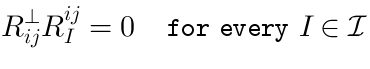
The exactness of the sequence (18) implies that the cohomology of (24) in fact coincides with the Lie algebra cohomology of the Lie algebra (22):

(25)

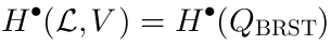
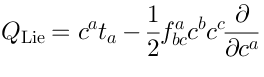
16 Lie algebra cohomology

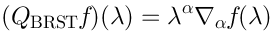
Lie algebra cohomology is well-known to physicists. Suppose that is a representation of the Lie algebra , with generators . The Lie-algebraic (usually called Serre-Hochschild) cohomology is the cohomology of the Faddeev-Popov operator:

17 Example: Maxwell theory

For example, consider the supersymmetric Maxwell theory in 10D in flat space. In the coset space approach, the flat space can be described as a group manifold of the Lie group , which is generated by supersymmetries plus Poincare translations.

Solutions of the equations of motion correspond to the ghost number 1 vertex operators. The BRST complex is based on the functions of and :
                
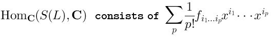
The space of functions (or, rather, the Taylor series) is dual to the universal enveloping algebra .

This is true for any group with the Lie algebra . The universal enveloping algebra can be identified with the left-invariant differential operators on of finite order, i.e. expressions of the form:
                
where . Then given a function on , we can compute the derivative of at the unit :
                
This requires the knowledge of the coefficients of the Taylor series of at .
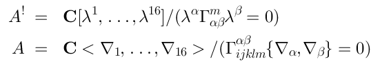
Therefore we observe the duality relation between the functions on and the elements of the universal enveloping algebra .

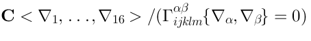
Therefore in this case:

(26)

Then Koszul duality (25) tells us that the space of vertex operators is:

(27)

The relation between and is the following:

(28)

where is some ideal.

This is just to say that the algebra “is a solution” to the Yang-Mills constraint:
           (*)
in the following sense. If we put — the generator of the supersymmetry transformation, then the constraint is satisfied. The definition (20), (22) of is such that is the most general (“universal”) Lie algebra satisfying this constraint; therefore any algebra satisfying the Yang-Mills constraint should be a factoralgebra of by some ideal.

The ideal can be described rather explicitly, in the following manner. Because of the quadratic relation (*), is proportional to :

(29)

(this is the definition of ). It turns out, as a consequence of (*), that:

(30)

So defined generates the ideal             

Simply put, this ideal consists of the elements of the algebra which vanish in the vacuum.

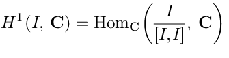
18 Using the Shapiro's lemma

One can show that:

(31)

In particular, the vertex operators (corresponding to ) are:

(32)

This formula may seem mysterious, but it has a transparent physical meaning. Indeed, it implies that the space of solutions of super-Maxwell equations is dual (as a linear space) to the space generated by and its derivatives .

This is what we expect: and its derivatives exhaust the gauge-invariant operators, i.e. gauge invariant linear functionals on the space of Maxwell solutions. Therefore:

This approach leads to the classification of gauge-invariant operators

Notice that automatically satisfies the Dirac equation:

(33)

19 Type IIB

We will now apply this method to Type IIB SUGRA.

We do not know what to do for a generic nonlinear SUGRA solution. This method (at least in its present form) can only be applied to the study of linearized fluctuations around the homogeneous space. But even this is technically nontrivial.

We will study the linearized excitations around a fixed background:

1. flat space

2. 

20 BRST complex

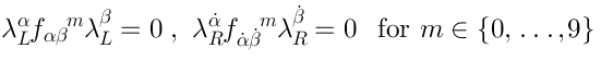
In Type IIB theory, there are two pure spinors and .

(34)

where are the structure constants of ,

The BRST complex computing supergravity excitations on the background is:

(35)

where is the space of polynomials functions of the order of two independent pure spinors and :

The space is the space of functions of and pure spinors , more precisely: Taylor series in and polynomials of the order in .

The is given by:

(36)

Here is the left multiplication by .

21 BRST complex

We want to have some description similar to Eq. (32) for Maxwell.

In Type IIB the role of is played by the Ramond-Ramond bispinor superfield . In flat space one can think about as the product of left and right ’s:

(37)

(but there are no such things as and ).

As we explained, in Maxwell theory the superfield was interpreted as the generator of the ideal , more precisely of its “abelianization” . Is there a similar interpretation in Type IIB?

It turns out that in Type IIB the situation is more involved.

We will answer this question for Type IIB in and in flat space. We will find an interpretation of the Type IIB gauge invariant operators in terms of an ideal in some infinite-dimensional Lie superalgebra which we will call .

But:

• will not be a quadratic Lie algebra

• this interpretation will come with a puzzle

22 Our stratedy

• Interpret the standard BRST complex as a Lie algebra cohomology complex for some infinite-dimensional Lie algebra; actually we will need the so-called relative Lie algebra cohomology

• This relative cohomology can be interpreted as the cohomology (usual, not relative; and with trivial coefficients) of some ideal, which is defined similarly to the ideal of the Maxwell theory

We can do this for both and flat space.

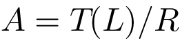
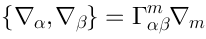
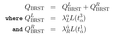
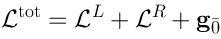
23 Definition of the Lie algebra

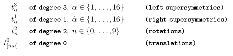
We will start with . We define the Lie algebra as a sum of two copies of , plus some finite-dimensional Lie algebra (as linear spaces):

                 (38)

which are all “glued together” as follows:

(39)

where is the structure constants of — the algebra of supersymmetries of .   Comments:

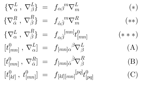
1. Our is not a quadratic algebra (because of Eqs. (A), (B) and (C))

2. Eq. (*) defines a quadratic subalgebra which we call , and Eq. (**) defines

3. Each and is the same as the Yang-Mills (or Maxwell) algebra (20)

4. The rest of relations tell us how to “glue together” and

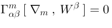
5. Eq. (C) tells us that the generators form — rotations around a point in

24 Relative cohomology

Consider any representation of . It is also a representation of :

is a representation of is a representation of      

Indeed, let us remember the structure of the . The generators are:
The subalgebra is generated by . To have a representation of means to have operators , , , acting in the linear space .
We then define the action of in in terms of the action of :

     

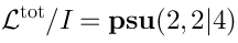
This is consistent. In fact, there is an ideal such that
We defined so that .

25 Relative cohomology

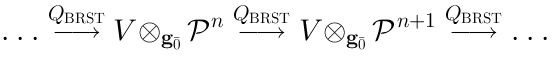
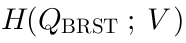
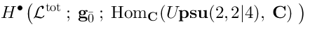
Let us consider the BRST cohomology:

(40)

where  .    The cohomology of this complex will be called:

(41)

---

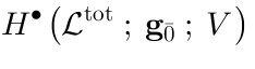
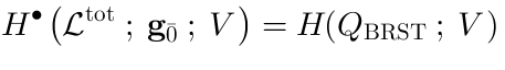
On the other hand, consider the relative cohomology group:

(42)

---

We claim that (42) coincides with (41):

(43)

In fact (41) is the usual (slightly generalized) BRST cohomology of the Berkovits formalism.
And (42) is a new description.

Let me explain why (41) is the usual BRST cohomology. Let us take as the space dual to the universal enveloping :

  (44)

On the RHS, we have acting on the space:

(45)

This is the space of sections (or rather, Taylor series of sections) of the pure spinor bundle over (was explained here). In other words, this is the “usual” BRST complex on the pure spinor worldsheet.

---

And now let us see what we have on the left hand side of (43).

26 Relation to the cohomology of the ideal

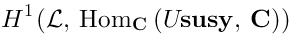
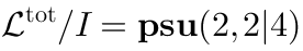
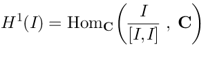
We now look at the relative Lie algebra cohomology:

(46)

There is an ideal such that:

(47)

This ideal consists of those combinations of the covariant derivatives which vanish in the vacuum . It turns out that the relative cohomology (46) coincides with the cohomology of :

(48)

The proof is in the paper.

We will therefore proceed to study .

27 Ghost number 1

The elements of correspond to the global symmetry currents of the -model. There are finitely many global symmetries. We have:

(49)

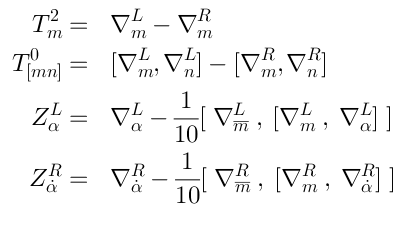
We will now show that is a finite-dimensional representation of , actually the adjoint representation of . How do we see this?

As a representation of , is generated by the following objects:

(50)

Remember are defined from and similarly .
The bar over index means:
        

We see that is a finite-dimensional space.

Why there are no more elements? For example, let us consider . Modulo this is same as , and using Eq. (39) this is proportional to .

Similarly, all the other covariant derivatives of every element of (50) can be expressed as a linear sum of other elements. Therefore, they form a closed representation of .

28 Ghost number 2

Ghost number 2 should correspond to the physical vertex operators:

(51)

We have only studied them in flat space.

As we will explain, there is a puzzle even in flat space.

It is more convenient to study the homology , instead of the cohomology. The relation between them is the Poincare duality:

(52)

The homology has a very straightforward elementary description. It consists of the elements of the form:

(53)

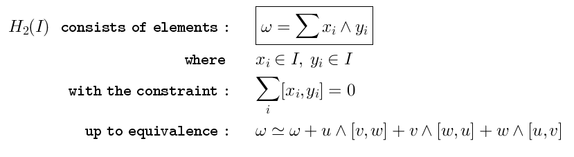
29 Ghost number 2

As in the case of Maxwell theory, elements of should correspond to the gauge invariant operators in Type IIB theory.

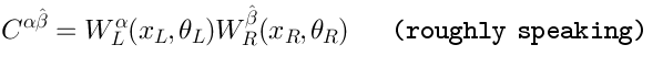
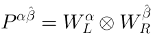
Let us consider the case of flat space. The simplest thing we can reproduce is the Ramond-Ramond bispinor:

(54)

Here is defined using the “left” part of — see Eq. (38). It automatically satisfies the Dirac equation, because and satisfy the Dirac equations (33).

30 Ghost number 2

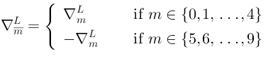
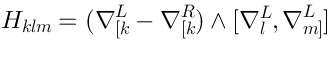
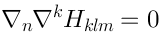
The NSNS 3-form field strength should correspond to:

(55)

It turns out that the linearized SUGRA equations of motion are not satisfied, because . However, the derivatives of are all zero:

(56)

therefore this is a “zero mode effect”.

This is a puzzle. Most likely, the zero modes are not correctly reproduced in the current version of the pure spinor formalism. The disagreement in the zero mode sector was discussed in arxiv:1005.0049 and arxiv:1203.0677. It would be useful to explicitly trace the connection between the nonzero and the “non-physical” vertex found in those papers.

31 Conclusions

The pure spinor formalism is now well-developed. But the Koszul duality was not widely used, at least not in the string theory literature. We tried to study this duality by applying it to the Type IIB supergravity, more specifically to the classification of the linearized excitations of homogeneous spaces. We had to invent a modification of the duality, which involves the “left” and “right” quadratic algebras glued together in some special way. This gives an elegant description of the ghost number 1 operators, and a puzzle for the ghost number 2 operators.

More research is needed in this direction.