Comparison to boundary S-matrix

Periodic array of operator insertions

Let and be two local operators, and and some c-number densities with support in sufficiently small compact space-time regions. Let us consider the following deformation of the action ( cf. Eq. (60)) :

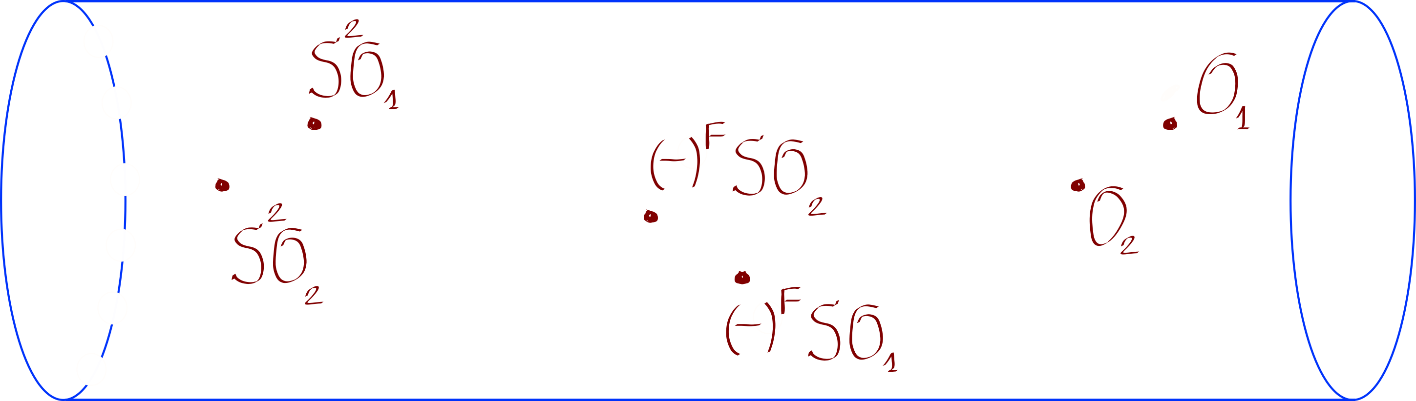Two periodic arrays of insertions

where and are two nilpotent coefficients. This is, essentially, an infinite periodic array (designed to satisfy Eq. (60)) of compactly supported deformations.

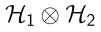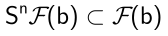
At the linearized level, i.e. assuming , the two terms in the deformation transform in two infinite-dimensional representations, and . But if we do not assume , then there will be a term in the SUGRA solution proportional to , and it will not transform in . We can consider the space of all possible completions of linearized solutions to nonlinear solutions. The terms proportional to form a linear space , which, as a representation of , is an extension:

Even if we restrict on , there are such nontrivial extensions. The corresponding cocycle:

is nontrivial, the average of over the period (see Eq. (18)) is nonzero.

Let us insert, instead of an infinite array, just two operators: and . Consider the “retarded” solution excited by them. The waves will keep bouncing from the boundary of AdS, interacting in the middle. Therefore the part will grow in global time like square of . We consider this a complication. To simplify the analysis, let us make four insertions (instead of just two):

Then the terms linear in , as well as the terms linear in , will cancel in the future. But, before they cancel, there will be some interaction, generating terms proportional to . In the future, the -terms become a solution of the free equation. This is the “retarted” solution generated by these insertions, i.e. the one which is pure 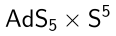in the past.

Monodromy vs boundary S-matrix

Let us suppose that is a delta-function at the point on the boundary, and delta-function at the point . Genarally speaking, every point on the boundary of AdS defines a Poincare patch, which can be defined as follows. Consider the future of , denote it (a subset of AdS). Notice that for any : . Consider the “first fundamental domain” of with respect to the action of , i.e. the set of points 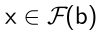such 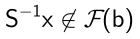. This is the Poincare patch corresponding to (the beige area on the Figure). For the retarded solution corresponding to the insertions (75) all the interaction happens inside .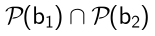

This implies that the average of , in the sense of Eq. (18) can be computed as the integral over . In fact, since the boundary-to-bulk propagator has support on the light cone, see Eq. (61), the integral is supported on . The integrand is the retarded propagator times triple-interaction vertex.

On the other hand, in the definition of the boundary S-matrix Witten:1998qj the integration of the interaction vertex is over the whole Euclidean AdS. It is not clear to us how these two definitions are related.

Normalizable and non-normalizable contributions to monodromy

Notice that goes all the way to the boundary, therefore there is no reason why the monodromy would be a normalizable solution. However, the non-normalizable part is due to waves bouncing back and forth in AdS reflecting from the boundary. Therefore all the non-normalizable terms can be damped by making adjustments, of the order , of the boundary conditions. In other words, correcting the defining Eq. (75) by adding some operators of the order . Then, the monodromy of the modified array will be a normalizable solution. We used this in Section Nonlinear beta-deformations have trivial monodromy.