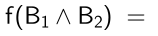
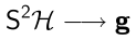
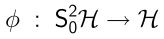
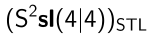
.
It does satisfy Eq. (
60).
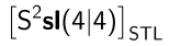
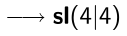
Linearized beta-deformations transform in the following representation:
where the subindex

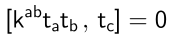
means zero internal commutator in the central extended

.
This means
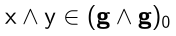
has
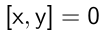
where the commutator is taken in
(
i.e. the unit matrix is not discarded).
It was shown in Aharony:2002hx that the renormalization
of beta-deformation is again a beta-deformation, and the anomalous
dimension is an expression cubic in the beta-deformation parameter.
We will conjecture that
the expansion of  starts with quadratic terms, and not with cubic terms.
This explains why the obstacle found in Aharony:2002hx is actually
quadratic rather than cubic.
starts with quadratic terms, and not with cubic terms.
This explains why the obstacle found in Aharony:2002hx is actually
quadratic rather than cubic.
But first,
in order to make contact with Sections Geometrical abstraction, Normal form of the action of  , Pure spinor formalism
we will discuss the description of the beta-deformation in the pure spinor formalism.
, Pure spinor formalism
we will discuss the description of the beta-deformation in the pure spinor formalism.
Description of beta-deformation in pure spinor formalism
Vertex operators of physical states live in

—
cochains of ghost number two.
The vertex corresponding to beta-deformation, as constructed in [
Mikhailov:2011si,
Bedoya:2010qz] is
actually not covariant. It transforms in

instead of Eq. (
63).
Some components of the vertex, transforming in

, are BRST exact:
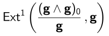
This defines a nontrivial extension, which can be characterized by a cocycle:
defining a nonzero class in
.
The existence of the commutative square formed by
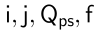
is nontrivial.
Then nontriviality is in the fact that

commutes with the action of
.
Generally speaking, the variation of
under the action of
could be non-zero, it just has to take values
in

. But there is a
-invariant
:
The composition

defines an element

, but
this group is zero by Shapiro’s lemma:
(Here

is the space of linear functions of pure spinors.)
Therefore exists

such that:
This means that the BRST-equivalent vertex:
Restriction of to even subalgebra
Let us start by forgetting about fermionic symmetries. In other words, consider the
restriction of
on the even subalgebra

.
Explicit computations of
Aharony:2002hx suggest
that
starts
with cubic terms,
i.e. with

(see Eq. (
9)) rather than

.
The
is certainly nonzero, and cannot be removed by the gauge transformations of Section
Gauge transformations.
This leads to an apparent contradiction. Indeed,
being non-removable means that it
represents a nontrivial class in:
But this cohomology group is zero, because
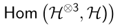
is finite-dimensional. The

of

with coefficient in a
finite-dimensional representation is zero —
see
FeiginFuchs.
What actually happens is:
where

is some infinite-dimensional extension of

.
We will now explain this.
Infinite-dimensional extension of finite-dimensional
The perturbative nonlinear solution involves terms proportional to
 in the notations of Appendix AdS notations.
These terms, under the action of
in the notations of Appendix AdS notations.
These terms, under the action of  and
and  (see Eqs. (33), (34)),
generate an infinite-dimensional representation. We will first explain the origin of -terms,
and then the structure of the infinite-dimensional extension of .
(see Eqs. (33), (34)),
generate an infinite-dimensional representation. We will first explain the origin of -terms,
and then the structure of the infinite-dimensional extension of .
Log terms
We will now explain the origin of at the third order in the deformation parameter.
Following
Aharony:2002hx, let us consider those linearized beta-deformations which
only involve the RR fields and the NSNS

-field in the direction of

. At the linear level, these
solutions do not deform

at all
.
At the cubic order, the interacting term has three linearized solutions combine in a term proportional,
again, to the beta-deformation of
. This means that we have to solve the equation in
:
Structure of
(Notations of Appendix
AdS notations.)
Consider, for example, a massless scalar field, whose
-dependence corresponds
to a harmonic polynomial

of degree

. There are solutions of the form:
where

is a harmonic polynomial of degree
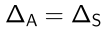
.
Such solutions generate a finite-dimensional representation

of
.
Now let us allow
to have denominators, either

or

,
keeping the same overall homogeneity degree
.
(It is important that

is never zero, in fact

.)
Then, the solutions (still given by Eq. (
65)) generate an infinite-dimensional
representation

of
. It contains a finite-dimensional subspace
corresponding to polynomial
. Therefore,
is an extension of
.
This extension is non-split
,
because there is no invariant subspace complementary to

.
We explained the construction of extension for the simplest case of the massless
scalar field. The construction for other finite-dimensional representations is the same.
Finite-dimensional involves scalar fields, tensor fields, and fermionic spinor fields,
and they all can be non-constant spherical harmonics on .
Importantly, for a finite-dimensional , all these fields are polynomials in  .
To extend to , we just allow negative power of or negative powers of
.
To extend to , we just allow negative power of or negative powers of  .
.
We would like to stress that all these extensions only contain rational functions of ,
with denominators powers of and . The perturbative solution contains
non-rational terms, e.g.  . But only has rational functions,
all logs got differentiated out.
In this sense is simpler than ( cp. Section is simpler than perturbative classical solutions).
. But only has rational functions,
all logs got differentiated out.
In this sense is simpler than ( cp. Section is simpler than perturbative classical solutions).
Example of cocycle
A nontrivial cocycle

in
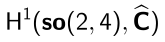
can be defined by the following formulas
(notations of Eqs. (
33), (
34)):
(In other words,

is the variation of

under

.)
Here

is the infinite-dimensional extension of the trivial
representations, generated by massless scalar fields allowing denominators powers of
.
Composing this
with some intertwining operators
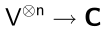
we may get nontrivial cocycles in

.
Renormgroup flow generates infinite-dimensional representations
We must stress that takes values in , and not in .
Of course, is contained in , as a subrepresentation.
But there is no invariant projector from to .
We can say that the renormgroup flow of the beta-deformation results in
the infinite-dimensional extension of the representation of beta-deformation.
The same is true for other finite-dimensional deformations. A renormgroup
flow of a finite-dimensional deformation generates infinite-dimensional extensions of
(possibly other) finite-dimensional representations.
This, of course, implies that we should also extend our space of linearized solutions.
We should start with
rather than just
. Otherwise, in the
notations of Section
Action of a symmetry in local coordinates,

will lead out
of (
i.e. not tangent to)
the image of

. Then, the coefficient of

in the expansion of
in powers of

lives in
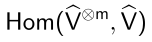
.
Nonlinear beta-deformations have trivial monodromy
We have an intuitive argument, that the monodromy always takes values in unitary representations.
Indeed, non-normalizable excitations can be thought of as waves bouncing back and forth from
the boundary of AdS. They can be all damped by emitting appropriate excitations from the
boundary, i.e. by adjusting the boundary conditions. Only normalizable modes remain.
(See Section Normalizable and non-normalizable contributions to monodromy.)
Suppose that the monodromy were nontrivial. Let us consider the lowest order in -expansion
where it be nontrivial. At the lowest order, it commutes with the undeformed action of .
Therefore, it must take values in a finite-dimensional representation (since the tensor product of
any number of is still finite-dimensional). But finite-dimensional representations
are not unitary.
This argument implies, more generally, that the monodromy of finite-dimensional deformations is identity.
In Section Comparison to boundary S-matrix we will consider infinite-dimensional deformations,
with nontrivial monodromy.
Lifting of to superalgebra
Let  be the part of
  (see Eq. (11)) involving only the ghosts
of even generators of
(see Eq. (11)) involving only the ghosts
of even generators of  (essentially, all the ghosts of odd generators all put to zero).
The
(essentially, all the ghosts of odd generators all put to zero).
The  of Eq. (64) is annihilated by .
What happens if we act on with the full , including the terms containing odd indices?
Can we extend to a cocycle of ?
of Eq. (64) is annihilated by .
What happens if we act on with the full , including the terms containing odd indices?
Can we extend to a cocycle of ?
To answer this question, let us look at the spectral sequence
corresponding to
FeiginFuchs
It exists for any representation
. At the first page we have:
Our
belongs to

. The first obstacle lives in
We actually know that the SUGRA solution exist. Therefore this obstacle automatically vanishes.
But there is another obstacle, which arizes when we go to the second page. It lives in:
We used the fact that relative
cochains are
-invariant, therefore the cocycles automatically fall into the finite-dimensional

. In fact, this obstacle does not have to be zero, because
there is something that can cancel it. Remember that
is generally speaking not annihilated
by
, but rather satisfies Eq. (
13). And, in fact, there is a nontrivial cocycle:
We conjecture
that the supersymmetric extension
of
indeed exists, but instead of
satisfying

satisfies:
We will now describe of Eq. (66).
Step 1: construct an element of

Consider an element of
corresponding
to the extension
:
(Remember that
is defined in Eq. (
63).)
Step 2: compose it with an intertwiner
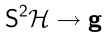
It was shown in
Bedoya:2010qz that there exists a
-invariant map
Construction of the intertwiner
We will now construct the intertwining operator in Eq. (68).
Algebraic preliminaries
Suppose that we have an associative algebra

. For any

consider their product:
In particular, take
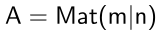
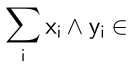
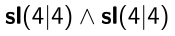
— the algebra of supermatrices. Let us view the exterior product

as a subspace in

.
For any element

we define:
We observe that:
Therefore, the operation

defines a map:
We degine the “split Casimir operator”:
where

are generators and

some coefficients, which we now define.
It satisfies:
In particular, if we think of generators as matrices:
In matrix notations:
Notice that for any matrix

:
We define:
Description of
In this language, the representation
in which beta-deformations transform consists of expressions:
Description of the intertwiner
For

and

belonging to
, we define:
The correctness w.r.to the equivalences relation of Eq. (
70) follows immediately.
It remains to verify the correctness w.r.to Eq. (
71). Indeed,
under the condition
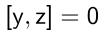
and

we have:
(We used Eq. (
69).)
Therefore, we constructed a well-defined intertwining operator:
where
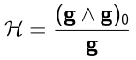
.
Intertwiner maps
to

Our intertwining operator
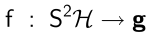
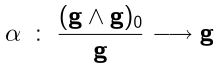
generates a short exact sequence:
and therefore a long exact sequence:
But

, therefore composition
with
is an injective map

.
We will now show that
,
i.e.
there are no intertwining operators. Suppose that there
is an intertwiner
Let us compute it on a decomposable element

.
Here

denotes the symmetrized tensor product.
The only way of contracting indices resulting in an antisymmetric tensor is:
antisymmetrized over both

and

.
(The terms like
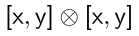
belong to

rather than

.)
But anticommutators are not allowed, because
should be correctly defined
with respect to
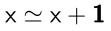
.
Structure of 
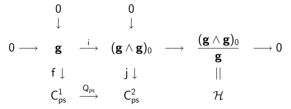
Let us denote:
the subspace of
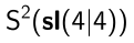
consiting of elements

such that
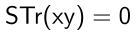
.
The map:
is an intertwiner. There is a map
The composition of the map of Eq. (
73) and the map of Eq. (
74), combined with the projector

,
equals to the map
of Eq. (
72):
By definition
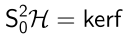
. This means that
has some invariant
subspaces:
This finer structure does not seem to be relevant for the leading term in the beta-function.
Role of in anomaly cancellation
Our construction of the cocycle as a product:
suggests that it participates in anomaly cancellation.
It was explained in [
Bedoya:2010qz,
Mikhailov:2012id] that at the level of the classical
sigma-model there is no reason for the parameter of the beta-deformation to have
zero internal commutator. From the point of view of the classical worldsheet, the beta-deformations
live in

, and not necessarily in
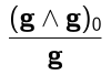
.
But at the quantum level, on the curved worldsheet,
the deformations with nonzero internal commutator suffer from one-loop anomaly.
This suggest the following anomaly cancellation scenario. Let us start with the linearized
physical (
i.e. with zero internal commutator) beta-deformaion, and start
constructing, order by order in the deformation parameter
, the corresponding nonlinear solution.
The classical construction goes fine, but at the secondr order in
we may encounter a one-loop anomaly
of precisely the right form to be cancelled by a non-physical beta-deformation. (“Nonphysical” means
with non-zero internal commutator.) Then, we just add, with the coefficient

,
some nonphysical beta-deformation, to cancel that anomaly.
But the subtlety is, that the extension of physical deformations by nonphysical:
is not split. In other words, it is impossible to lift
back to

in a way preserving symmetries. In this sense, the anomally may break global symmetries.
In our language this means that the nontrivial
of Eq. (
9) may be
induced by quantum corrections at the first order in

.
But our conjecture is that the nontrivial is present already at the classical level
and its cohomology class participates in Eq. (66).
Both conjectures have to be settled by explicit computations, which we have not done.
Outline of computation
We believe that the best framework for actually computing
and proving the conjectured
Eq. (
67) is the pure spinor formalism. This can be done using the
homological perturbation theory developed in [
Bedoya:2010qz,
Benitez:2018xnh]. The basic idea is to consider
the deformation of the pure spinor BRST operator:
The explicit expression for

was obtained in [
Bedoya:2010qz,
Benitez:2018xnh]. The next
step is to find

such that

is nilpotent up to terms of the order

.
This was done in [
Bedoya:2010qz,
Benitez:2018xnh], but only for a special class of deformations (essentially,
those leading to the integrable model, see [
Berenstein:2004ys,
Bundzik:2005zg,
Klimcik:2008eq,
Delduc:2013qra,
Hollowood:2014qma,
Hoare:2015wia,
Benitez:2018xnh]). The deviation from
-covariance would arise for
non-integrable deformations,
i.e. those cases where the

was
not found in
[
Bedoya:2010qz,
Benitez:2018xnh].
Other finite-dimensional deformations
Besides beta-deformations, there are infinitely many other finite-dimensional
deformations [Mikhailov:2011af,Mikhailov:2017uoh].
The formalism developed in this paper should be also applicable to them.


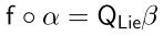
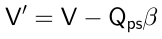


is a compact manifold. Indeed, the NSNS
-field is a two-form. Nonzero harmonic two-form cannot exist on a compact manifold. But in fact, because of the undeformed
has the RR five-form turned on, the linearized equations actually mix RR with NSNS fields, leading effectively to massive equations.

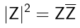 . Denominators
are powers of
. Denominators
are powers of  only enter polynomially.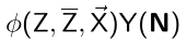
and another allowing
. But we want to keep the real structure, so we must combine them.

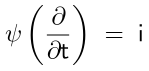
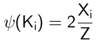
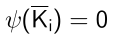

on the lifted solutions does not lead out of the space of lifted solutions
where
is some angular coordinate of
being a linear function of
, i.e.
). The simplest solution is
. It has nontrivial monodromy
. But we can add to it the expression
which is annihilated by
and cancels the monodromy. In general, exists solution with all logs being
, no monodromy.

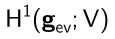








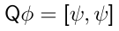
is
; it corresponds to the extensions Knapp of
by
.

 .
.
, there is a natural action of the symmetric group
on the tensor product
. For example, when
, the transposition
acts as:
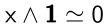
. The exterior product
is the subspace of
.