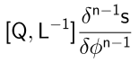
Relation to tree level Feynman diagrams
Here we will apply the formalism of Section Obstacles to linearization of symmetry to the case when
 is the space of solutions of some classical nonlinear field equations, constructed
as perturbation of some zero solution
is the space of solutions of some classical nonlinear field equations, constructed
as perturbation of some zero solution  . This is
different from the context of deformations of QFT ,
but the AdS/CFT correspondence establishes a relation between these two contexts (Section Supergravity in AdS space).
. This is
different from the context of deformations of QFT ,
but the AdS/CFT correspondence establishes a relation between these two contexts (Section Supergravity in AdS space).
Perturbation theory as a map 
Let us take
to be the space of perturbative solutions

of nonlinear equations of the form:
where

is some linear differential operator, and

is a nonlinear function
describing the interaction. We assume that

is a polynomial starting with
the terms of quadratic or higher order.
The point
will be the zero solution

.
Then

can be identified with the space of solutions of
the linearized equation:
Tree level perturbation theory can be thought of as a 1-parameter map
parameterized by a small parameter

. As explained in Section
Geometrical abstraction,
it can be also understood as a map
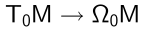
.
We will embed
into the space

of all field configurations,
not necessarily satisfying equations of motion (subindex “os” means “off-shell“).
We assume that
is a linear space. We consider

as a function
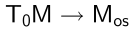
. It can be described as a sum of tree level Feynman
diagrams. Every incoming leg corresponds to a solution of the linearized equation
(
21). Every internal leg and the outgoing leg each correspond to a propagator

.
There is a recursion relation
:
where
satisfies:
The definitions of the operator
has an ambiguity
(because one can add a solution of the free equation). Suppose that we made some choice of
.
The dependence on the choice of
is controlled by Lemma
27 below.
As we already explained, we need an embedding of into the linear space of
off-shell field configurations , just because we want to add Feynman diagrams.
Obvously, the space of free solutions is also embedded into .
Let us assume that the action of  on agrees with this embedding.
This is not really important, but we make this assumption for this Section.
For example, suppose contains time translation
on agrees with this embedding.
This is not really important, but we make this assumption for this Section.
For example, suppose contains time translation  .
We assume that it acts as
.
We assume that it acts as 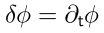 , both on and on .
Let us define

as follows:
(the dependence of

on the RHS comes from

).
Lemma :
This is the same as defined in Eq. (12):
Proof We have to show that for any

.
In other words, for any

:
We will use:
We have:
Together with Eq. (
26) this implies:
The proof can be put in slightly different words, as follows. Notice:
Every time
hits

, we get

:
—
this gives the

term on the LHS of Eq. (
25). And when
hits one of the
,
we get
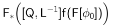
.
Lemma :
An infinitesimal variation of
:
where

satisfies
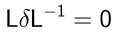
,
corresponds to an infinitesimal gauge transformation of
(see Eq. (
15)) where:
Proof
Amputation of the last leg
We will now present a slightly different point of view on the construction.
Suppose that for every linearized solution
we constructed a nonlinear solutions
(depending on a small parameter
). What should we do with
, to obtain

?
Remember that
is a (nonlinear) vector field on the space of
linearized solutions. Obviously, we have to somehow “project”
to a linearized solution.
According to Eq. (
24) we should remove the last leg, and replace it
with

:
Remember that
satisfies Eq. (
23):
Let us define the “amputator”

as the composition:
(Notice that

is a projector to

.)
It satisfies
:
If
is our perturbative solution (
i.e. 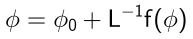
), then:
Trivial example
Consider a vector field
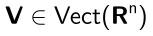
.
Suppose that

vanishes at

, and the derivative of
also vanishes at

:
Consider the following equation:
Let us construct solutions perturbatively in the vicinity of the constant solution:
For any functions

, we can expand it in Taylor series around

. We define
as follows:
The map

of Eq. (
22) is:
We observe:
According to Eq. (
24), to construct
we have to
take

and hit it with
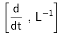
, which, according to Eq. (
29) amounts
to put
.
Therefore, in this case:
The gauge transformations of Eq. (
15) are:
where
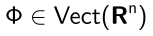
is another vector field.
Therefore, in this case the MC invariant computes the normal form of the vector field
(
i.e. modulo nonlinear changes of coordinates).
In this example we had  , and the structure of the first cohomology
group was rather tautological:
, and the structure of the first cohomology
group was rather tautological:  was the space of -invariants in .
In the next example we will consider the non-abelian
was the space of -invariants in .
In the next example we will consider the non-abelian 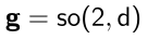 ,
with much more interesting (smaller!) cohomologies.
In particular,
,
with much more interesting (smaller!) cohomologies.
In particular,  can be nonzero only for infinite-dimensional
  .
.
Example: classical CFT on 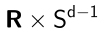
Consider a conformally invariant classical theory on the Lorentzian , for example
the  theory,
  .
.
Realization of as the base of the lightcone
Consider the light cone in

(
cp Eq. (
76)):
A convenient model for the conformal
is the projectivization of the light
cone, which is parametrized by
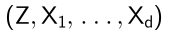
satisfying (
30) modulo the
equivalence relation:
A density of the weight

is a function

satisfying:
modulo functions divisible by

. Let

denote the space of such densities. The
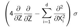
conformally invariant d’Alambert acts as follows:
This operator is only well-defined with this value of
, because for other values
of
it would not annihilate modulo
those functions which are divisible by
.
The elements of the kernel of
,
i.e. the solutions of free field equations, are
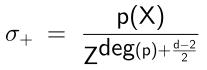
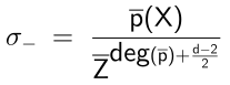
real sums of positive and negative frequency waves:
Conformal symmetry
Besides the rotations of

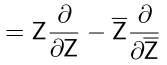
, there are also the following conformal
transformations:
Amputator
Introduce the Lie algebra cocycle

:
Consider elements of

periodic in global time. Any such element can be written as:
where the summation is over a pair of integers

and

is a
harmonic polynomial of
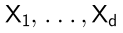
of the following degree:
We define
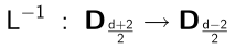
as follows:
Therefore:
These formulas
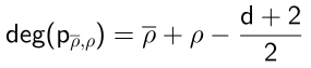
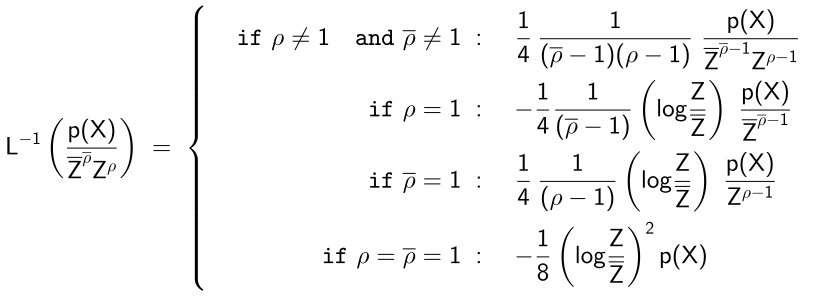
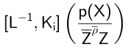
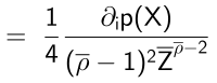
partially define a cohomology class
of Eq. (
35). The definition
is only partial, because Eq. (
36) does not describe all elements of
,
but only those periodic which are periodic in the global time
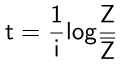
.
Generic elements are linear combinations of:
To completely specify
, we have to define
on elements containing powers of

, and compute
for them the commutators, as in Eqs. (
38), (
39), (
40). We will not do it here.
Relation to renormgroup
Our discussion of the classical field theory solutions in this section is a warm-up.
However, it
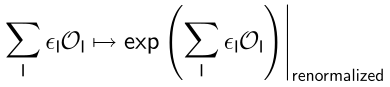
is related to renormalization. Given a set of operators

,
e.g. 
,
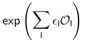
and a set of infinitesimal coefficients

, let us define the coherent state, schematically:
which in the classical limit corresponds to a classical solution.
This, of course, requires regularization. Therefore, the map
does not commute with the action of the symmetries. What we studied in this section
must be the classical limit of this map. This requires further study.
Comments on the structure of
is simpler than perturbative classical solutions
Let us continue with the example of the previous section.
Generally speaking, a perturbative solution is a sum of expressions of the form:
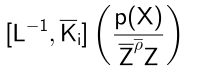
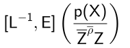
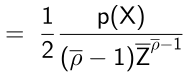
However, after the replacement of the last leg with
of eq. (
35), the resulting expression
does not contain “bare”
(
i.e. only contains
via its exponentials).
Indeed,

is
a solution of the free field equations. Solutions of the free field
equations do not contain powers of
. They only involve expressions of the form Eq. (
31).
No powers of
. In this sense, the amputated
is much simpler than full perturbative solution.
Moreover, we know that satisfies a constraint: the Maurer-Cartan Eq. (13).
In some situations, this might allow for some partial bootstrap, see Section Can be bootstrapped?.
There is a price to pay: the definition of contains an ambiguity. We could
have choosen a different . This corresponds to the gauge transformation of Eq. (14).
Moreover, the condition of -covariance is complicated:
The condition of -covariance is complicated
( cp Section Symmetries)
Under the false impression that all non-covariance is due to the “resonant” factors

, one might conjecture that

is

-covariant in
the sense that:
This, however, is not the case.
At least when
is a semisimple Lie algebra, Eq. (
44) is incompatible
with the MC equation:
because
takes values in vector fields of degree 1 and higher.
A semisimple Lie algebra cannot be represented by the vector fields
of degree 1 and higher. In fact, it follows immediately from Eqs. (
38), (
39) and (
40) that with

chosen as in Eq. (
37)

is zero when

is an infinitesimal rotation of
. This already contradicts Eq. (
44).
Instead of simple but wrong Eq. (44) we have more complicated Eq. (19).
Can be bootstrapped?
Consider an infinitesimal

-preserving deformation

of the action which is a monomial
of the order

in the elementary fields.
Then the corresponding cocycle,
representing a class of

, is given by the expression:
Could it be that
all is exhausted
by the expressions of this form for various
-preserving deformations?
This is certainly
not true for SUGRA on
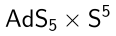
.
But in the situations when this is true, Eq. (
13) allows to recursively compute
, modulo
gauge equivalence described in Section
Gauge transformations,
starting from the terms of the lowest order in
given by Eq. (
45).
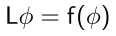


; remember that we assumed that

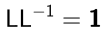


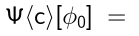
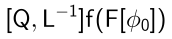










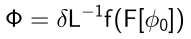
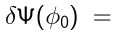




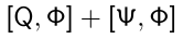

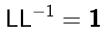


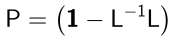
, where
and
, is nilpotent; the nilpotence of
is not necessary for the nilpotence of
.


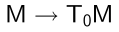 (Section Action of a symmetry in local coordinates), the inverse of
  . Then, again,
  .
.
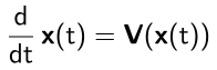
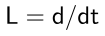 .
This equation is invariant under translations of
.
This equation is invariant under translations of 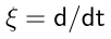 .
.



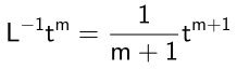



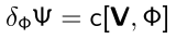
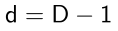
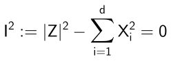



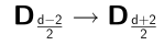





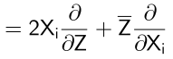

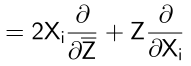




 ,
the corresponding solution of the MC Eq. (13) is:
,
the corresponding solution of the MC Eq. (13) is:
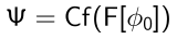
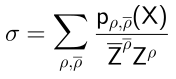



(Eq. (41)). But we know in advance that the resulting expression will not contain any powers of